Everything you need to know about multi-object tracking

I find Multiple object tracking (MOT) a very interesting problem. In the case called tracking-by-detection, you have a bunch of detections of objects (they can either be in 2D or 3D) and you have to associate detections in time figuring out if they are observation of the same object.

More formally, we can define the problem as a multi-variable estimation problem.

Given a set of frames, we have a set of states of objects in each frame. Let's call \(s_j^{i}\) the state of the object \(i\) in frame \(j\), all the \(M_j\) objects in the \(j\)-th frame are the set \(S_j = \{s^{1}_j, s^{2}_j, ..., s_j^{M_j}\}\). The set of the states \(S_{1:t} = \{S_1, S_2, S_3, ..., S_t\}\), defines all the states for all the objects in the frame sequence.

Now we have a set of observations for each frame \(O_{1:t} = \{O_1, O_2, ..., O_t\}\), where \(O_j = \{o^{1}_{j}, o^{2}_{j}, ... o^{M_j}_{j} \}\) are all the observations for frame \(j\). Note that for the sake of the notation we are assuming that we have exactly one observation for every and each object, \(M_j\) states and \(M_j\) observation at frame \(j\).

Now the problem that we want to solve is to find the "optimal" sequence of states given the observations. This can be solved as a maximum a posteriori estimation (MAP) problem

\[\hat{S}_{1:t} = \text{argmax}_{{S_{1:t}}} P(S_{1:t}| O_{1:t})\]

Usually, this can be solved either with a probabilistic approach or with an optimization approach. The former usually works online (more on this later) the latter is usually more suited for offline tracking since you want to optimize and find the global optimum on the whole frame sequence. This approach is also known as non-causal since you are using the future and past observations at the same time.

Probabilistic approach

Usually, to solve the problem with a probabilistic approach you can adopt a two-step iterative process:

1. you predict the state at the next step without using the observations (predict)
2. you correct your prediction with the observations (update).

To perform the predict step you need some dynamic model that you can use to compute predictions. To perform the update step you need some measurement/observation model that ties the observations back to the state so that you can perform the correction.

More formally:

\[ \textit{Predict}: P(S_t|O_{1:t-1}) = \int P(S_t|S_{t-1})P(S_{t-1}|O_{1:t-1})dS_{t-1}\]

\[ \textit{Update}: P(S_t|O_{1:t}) \propto P(O_t|S_t)P(S_t|O_{1:t-1})\]

Where \(P(S_t|S_{t-1})\) is the dynamic model that tells us how the states are supposed to evolve in time, and \(P(O_t|S_{t})\) is the measurement model.

Note that to be able to formulate this solution to the problem, we are assuming that the Markov assumption holds (past and future are independent given the current state).

Pros

• Works online.
• Can be less heavy computationally.

Cons

• Might not provide a global optimum, since we are not using the whole sequence.

Optimization approach

A second approach is to solve the estimation problem via optimization either of the Likelihood or minimizing an energy function.

More formally

\[ \hat{S}_{1:t} = \text{argmax}_{S_{1:t}} P(S_{1:t}| O_{1:t}) = \text{argmax}_{S_{1:t}} L(O_{1:t} | S_{1:t})\]

or considering an Energy function

\[ \hat{S}_{1:t} = \text{argmax}_{S_{1:t}} P(S_{1:t}| O_{1:t}) = \text{argmax}_{S_{1:t}} E(S_{1:t} | O_{1:t})\]

Note that models and in general knowledge about the expected behaviour of the objects can be injected also in the optimization approach. One very used approach is to enforce motion constraints through the function E.

Pros

• Converge to a global optimum.

Cons

• "Heavier" computationally.
• Works offline (you are using the future).

The Models

Let's talk a bit about the models which I find to be a very interesting aspect of MOT.

You have two problems to solve

1. how to measure the similarity between objects across frames
2. how to use that similarity information to recover identity across frames.

Roughly speaking, the first problem involves usually modelling the appearance or the motion of an object. While the second is the inference problem. Appearance here is used as a generic term, that could be the visual appearance if you are using a camera.

Two widely used approaches for modelling in MOT are appearance models and motion models. The former uses how an object appears to the sensor, the latter uses the expected motion of the object.

Let's have a look at examples, one of the simplest motion model consists of assuming that from one frame to the other an object didn't move much. If I have an observation in the frame \(j\) and I have a "close" observation in frame \(j+1\) I will associate them to the same object. What does close mean? I can for example measure the distance between the centroids, or I can use intersection over union, that is if the two boxes intersect more than a certain threshold they are matched in time.

This is a pretty simple approach that works. The main problems come from occlusions and the assumption (which might not hold) that the rate at which frames are captured it's "high" enough to capture very small motions in the observations. In the case of occlusions, you will likely experience id switches. This is given by the fact that boxes of different objects will overlap for some frames.

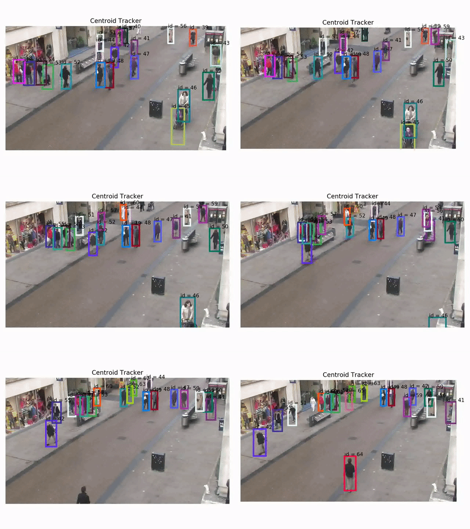
Let's see how a centroid tracker behaves for example. These results are obtained using the Oxford Towncentre Database for pedestrian tracking.

Detections are already available to be used for tracking.

As you can see the tracker works, but there are cases where id switch does happen, especially when the scene gets more crowded.

Now, if we want to make the tracker more robust we could either use an appearance model and use information about how the detected object looks or use a motion model and make assumptions about the motion of the detected objects (e.g., in the case of a pedestrian we can assume that the object will move with constant velocity).

Appearance models

Appearance models include two components:

1. a representation of the object appearance
2. a measurement of the distance between such two representations

In the case of visual tracking, lots of different representations can be used, such as local features (or deep features) of the image, colour histogram, HOG, etc...

In general gradient-based features, like HOG can describe the shape of an object and are robust to lightning changes, but they cannot handle occlusion and deformation well. Region covariance matrix features are more robust as they take more information into account, but they are more computationally expensive.

The distance between two representations can be computed in several ways, mainly depending on the appearance model used.

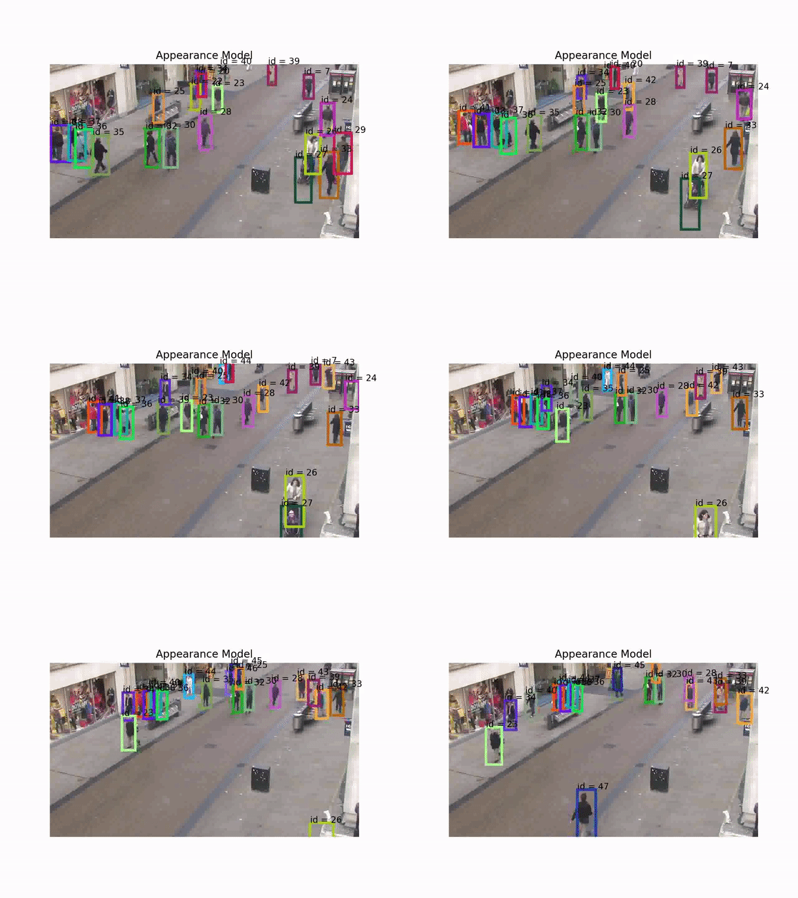
Let's see how our tracker improves using an appearance model.

As you can see the tracker is more robust to occlusion. This is given by the fact that we are using information about the appearance of the tracked objects so we don't "confuse" it with a different occluding object.

Motion Models

As a final topic let's have a look at motion models. Motion models assume knowledge about how an object moves and predict the expected position of the object. The predicted position is later corrected and updated with the measurement, which is now matched to the predictions.

A very common way to use motion models in the probabilistic iterative approach is to use Kalman Filters. A very common assumption is that the objects move with constant velocity or constant acceleration.

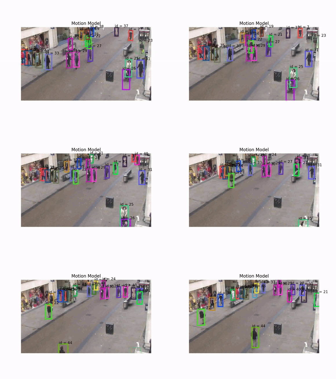
Let's have a look again at how using motion models improves our tracker.

Here we are using a Kalman Filter with a constant velocity model. The tracker is still robust to occlusion since we are predicting the future position of each object using the motion model.

The models solve the problem of how to measure similarity, the second problem of using the similarity to recover identity can be solved in several different ways. In the presented demo cases, it was solved by optimization of the intersection over union between the tracker tracks after the update and the observations.

The examples were created using modified versions of tracking code from this repository.

---

Conclusions: We had an in-depth look at the multi-object tracking problem, how it can be formalized formally and solved. We had a look at some classic ways of solving it and we also had a look at the real-life example of pedestrian tracking