Re-identification with Triplet Loss

One very interesting computer vision problem is re-identification. The idea is that you have images of some entity and you want to be able to re-identify that entity in new images. As a complementary problem, you might also want to be able to say if an identity is known or not.

Classic use cases are people re-identification for surveillance, but there are also more fancy use cases such as whale re-identification for monitoring and conservation effort.

A classic way of solving the re-identification problem with Deep Learning is to train a CNN to learn an embedding space where different observations of the same entity will be mapped close together, or better closer than observation of a different entity.

Formally this approach, called learning metric embeddings, has the goal of learning a function that takes images in a space \(R^{F}\) to a space \(R^{D}\) where semantically similar points in the initial space are mapped to metrically close points. At the same time, semantically different points in the original space are mapped to metrically distant points.

What we want to learn it's the function

\[\textit{f}_\theta(x): R^{F} \rightarrow R^{D}\]

The function is usually parametric and can be anything from a linear transform to complex non-linear maps.

A way to tackle the problem is to train a neural network to learn that function. In this case, we can use one of the final layers of the network as the embedding space, we just have to come up with a loss function.

A typical approach at this point is to use a loss function that pushes points belonging to the same entity close togheter while pushing points belonging to different entities far away.

Let's define a metric \(D_{x, y}: R^D \times R^D \rightarrow R\) that measures a distance between the points \(x\) and \(y\) in \(R^D\).

In [1] the author proposed a loss function called Triplet Loss. The function is called triplet because it computes the loss over a triplet of points:

• the anchor \(x_a\), which is a sample of one entity
• the positive sample \(x_p\), which is another sample of the same entity used as anchor
• the negative sample \(x_n\), which is a sample of a different entity.

The function mathematically is:

\[ L = \sum\limits_{a,p,n}[m + D_{a,p} - D_{a,n}]_+\]

where \([\bullet]_+\) it's the hinge function \(max(0, \bullet)\).

It is pretty straightforward to see that the loss is pushing the distance function \(D\) between the anchor and the positive sample closer to the distance between the anchor and the negative sample by at least a margin \(m\).

Usually, the Euclidean distance is used as the metric \(D\).

A modification can be made to the Triplet Loss to introduce what is called a soft margin. In this case, the hinge function is modified to be

\[\text{softplus} = log(1+e^x)\]

This yields mainly two advantages:

1. we remove one hyperparameter (\(m\))
2. the softplus function decays exponentially instead of having a hard cut-off like the hinge function. This means that triplets that already satisfies the margin \(m\) will still contribute a bit to the loss with the effect of still pushing/pulling samples as close or as far as possible.

Ok so let's give this a try in a real re-identification case.

A real-life re-identification problem

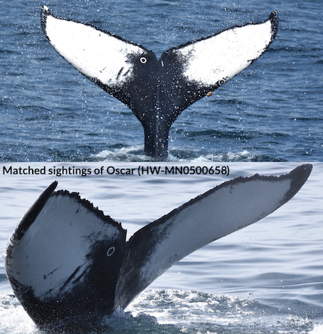
Let's use as a test case the whale identification task from last year Humpback Whale Identification Kaggle competition. The task for the competition was to train a model able to identify a whale by their fluke (which is unique for each whale, kind of like a fingerprint). This is a nice real-life case, the dataset it's unbalanced, noisy and there are lots of nuances:

• it's not easy to take consistent pictures of moving flukes, so you will have a wide variety of viewpoints and occlusions (mainly water splashes)
• flukes can slightly change in time due to injuries

Just for reference, that's what the images look like.

The full code for our experiment can be found here.

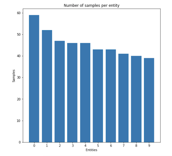
To simplify the problem, let's use a smaller dataset consisting of only the 10 whales with the highest number of occurrences. The histogram of the sample count for this smaller toy dataset is shown below.

For the task, we will use a pre-trained Resnet34 as the main feature extractor and we will add a final linear layer with \(D=128\), which will be the dimension of our metric space.

Let's see how the embeddings evolve in 2D during training, each colour represents a different whale.

How do we evaluate now our network?

Since we used the Euclidean distance, a solution it's to compute the embeddings for the validation set, for each of them find the nearest embeddings of the training set and use that information to infer the entities in the validation set. For the sake of this example, I just computed classification accuracy, assigning to each validation sample the label of the closest training sample.

I used the accuracy as the monitor variable for early stopping. After 55 epochs we got an accuracy of 0.93.

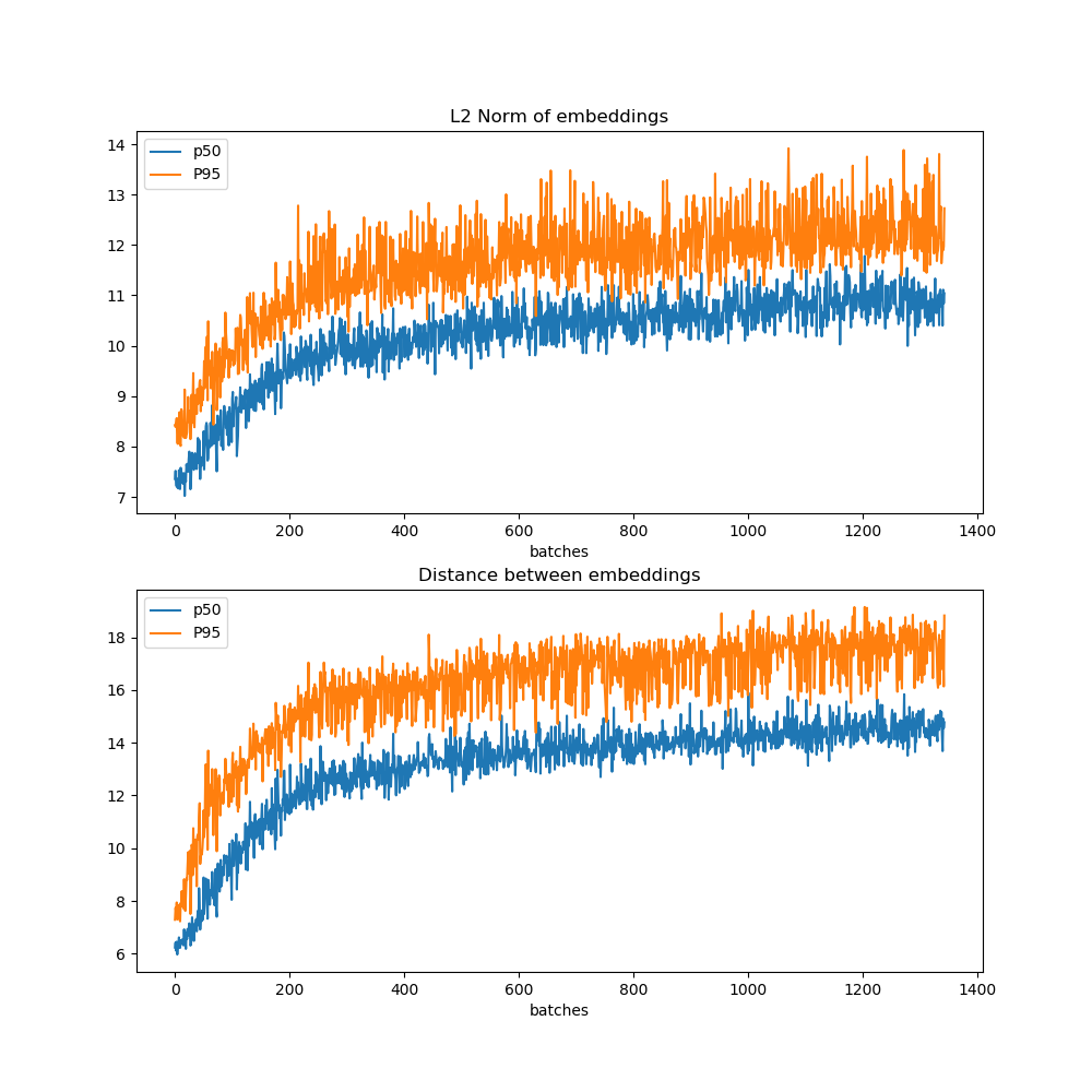
Some interesting variables to monitor while training for metric learning using the Triple Loss are the norms of the embeddings and the distances between embeddings. Let's have a look at the median and the p95 of those quantities as they evolve for any mini-batch.

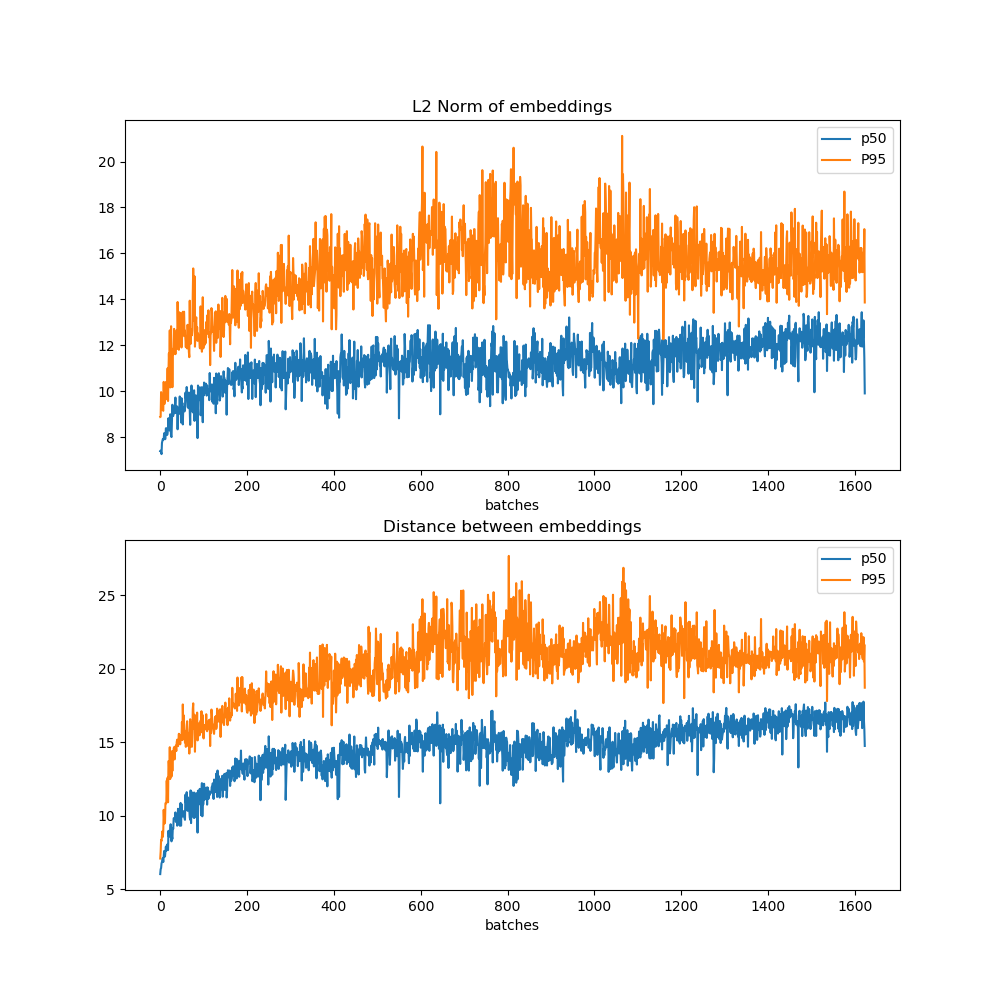
As you can see, as the training proceeds, the embeddings are pushed to become larger and larger and be more and more distant between each other. These plots are also really informative to decide when to stop the training (more on this later).

Can we do better?

If you think about how we trained the network, we randomly got anchor samples, for each one of them we randomly selected positives and negatives. What usually happens is that the network learns quickly the easy triplets which start to be uninformative during the training process. A solution to this would be to present all the possible combination to the network during the training process, but that can become impractical as the number of samples grows.

The problem can be solved "mining" for hard triplets. What's a hard triplet?

A triplet can be defined hard when \(D_{a, p} > D_{a, n}\), that is the negative is closer to the anchor than the positive. Those are the triplets that need the biggest correction.

We have two ways of mining triplets, offline and online.

Offline triplet mining

We compute all the embeddings at the beginning of each epoch and then we look for hard (or semi-hard triplet when \(D_{a, n} - D_{a, p} < m \)). We can then train one epoch on the mined triplets.

Mining offline it's not super efficient, we need to compute all the embeddings and update the triplets often to keep our network seeing hard examples.

Online triplet mining

In online mining, we compute the hard triplets on the fly. The idea is that for each batch, we compute \(B\) embeddings (where \(B\) it's the batch size), we now use some smart strategy to create triplets from these \(B\) embeddings.

An approach called batch hard was proposed in [2], where you select the hardest positive and the hardest negative triplets in the batch.

1. Select for each batch \(P\) entities and \(K\) images for each entity (usually \(B\leq PK \leq 3B\)).
2. For all the anchors find the hardest positive (biggest \(D_{a,p}\)) and the hardest negative (smallest \(D_{a, n}\))
3. Train the epoch on the mined hardest triplets.

As a note on \(P\) and \(K\) size. \(3B\) it's the number of embeddings we would have to compute while mining offline. To get \(B\) unique triplets you will need \(3B\) embeddings.

There are lots of practical considerations to be made with this approach, for example:

• Is the dataset clean? Are the hardest triplets impossible triplets that are just confusing the network?
• In some cases you might not have \(K\) samples for each instance (few-shot learning), or you might have only 1 (one-shot learning). In this case, augmentation might be your friend. If you can heavily augment the samples you could use the same images to reach \(K\).
• Overall, it might be a good idea to do a first round of training without mining to bootstrap the network and then later switch to hard triplets mining.

Still each use case it's different, so the best thing to do it's experimenting.

Ok, let's retrain using hard batch online mining and let's see how our network behaves.

After 47 epochs, our training stopped reaching 0.95 accuracy.

This is the embeddings evolution during training.

Let's have a look again and the evolution of norms and distances of the embeddings.

In this case, it is even more relevant to have a look at the distance/norm plots to decide when to stop training. What can happen is that the loss my appear stagnating, since as soon as the network has learnt hard cases, new ones will be presented. For example, looking at the graph we could have probably trained the model more.

Another useful number to be checked to see how training is going it's the number of active triplets, that is the number of triplets with non-null loss.

---

Conclusions: We had an in-depth look at how to solve the re-identification problem using Deep Learning. We understood the triplet loss and how it can be improved using triplet mining. We had a look at a real-life re-identification example and solved it with the concepts we learned.

[1] FaceNet: A Unified Embedding for Face Recognition and Clustering

[2] In Defense of the Triplet Loss for Person Re-Identification