The eight-points algorithm
In this blog post we had a look at how to estimate the optical flow (e.g., track how pixels move in time) in a set of images. The estimation we obtained gave us pixel matches across the image set.
Given the correspondences between two images, we can estimate the motion and the 3D position of the points we are observing. Solving this problem is known as Structure from Motion (SfM).
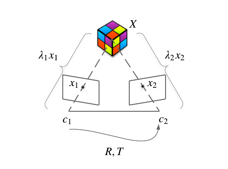
Let's assume we are observing a 3D point \(X\), in two different images. The two viewpoints are related by an affine transformation (rotation plus translation) given by the matrix \(R\) (for rotation) and by the vector \(T\) for the translation. If we draw an imaginary line between the image centres \(c_1\) and \(c_2\) to the 3D point, we have that the point is projected to the point \(x_1\) (in image space) in the first image and to the point \(x_2\) (in image space) in the second image.
In the camera frame, we can also write that \(\lambda_1 x_1 = X\) and that \(\lambda_2 x_2 = X\), being \(\lambda_1\) and \(\lambda_2\) the scaling factors to go from the points in the image to the point \(X\).
So, let's say that we know \(x_1\) and \(x_2\) (one of the matches we found between the two images), how can we recover \(R\), \(T\) and \(X\)?
Let's try and rewrite everything in the second camera frame.
\[ \lambda_2x_2 = R\lambda_1 x_1 + T\]
We can multiply for the skew-symmetric matrix of T
\[ \lambda_2 \hat{T}x_2 = \lambda_1 \hat{T}Rx_1 \]
we can then multiply for \( x_2^T \) and divide by \(\lambda_1\)
\[ x_2^{T}\hat{T}Rx_1 = 0 \]
Note: the term on the left gets to zero because \( T \times x_2\) is orthogonal to \(x_2\) so if you compute the scalar product for \( x_2 \) you get zero.
Now we have an expression that couples the camera motion and the two known 2D locations. This equation is called the epipolar constraint. Note that the 3D points \(X\) do not appear in the equation, we successfully decoupled the problem of computing \(R\) and \(T\) from the problem of computing the 3D coordinates of \(X\).
Geometrically, the epipolar constraint says something pretty straightforward. If you look at the first picture: the volume spanned by the vectors \(x_2\), T (\(\vec{o_2o_1}\)) and \(Rx_1\) (which is \(\vec{c_1x_1}\) seen from the second camera) has a zero volume, thus the triangle \((c_1c_2X)\) lies on a plane.
The epipolar constraint can be rewritten as:
\[ x_2^{T}Ex_1 = 0 \]
\(E\) is called the essential matrix, and it has the following property:
\[eig(S) = (\sigma, \sigma, 0)\]
That is the essential matrix has three eigenvalues, two are equals and one is zero.
\(R\) and \(T\) can be extracted from the essential matrix. Usually what we do in practice is that we find a matrix \(F\) that solves the epipolar constraint and then we compute the "closest" essential matrix (projecting \(F\) to the space of the essential matrices).
The eight-points algorithm
To solve the equation in \(E\) we need to re-write it in such a way to separate known variables (\(x_1\) and \(x_2\)) from the unknown \(E\).
If we stack the columns of \(E\) in a single vector \(E^{s}\) and we use the Kronecker product of \(x_1\) and \(x_2\) (\(a\)) we can write
\[ x_2^TEx_1 = a^{T}E^{S} = 0 \]
Now, we can stack this equation for all the matches we have between the two images and obtain the following linear system which contains all the epipolar constraints for all the points
\[ \chi E^{S} = 0 \quad \text{with } \chi = (a^{1}, a^{2}, ..., a^{n})^{T} \]
You can immediately see that the solution to the system is not unique and that every scaling factor multiplying \(E^{s}\) will solve the equation. In practice, this means that we are not able to compute the baseline, that is the translation between the two cameras, but only its direction. The solution is to consider the baseline equals to one and compute everything in "baseline units".
To have a unique solution at this points we need at least 8 points (that's what gives the name to the algorithm)
Once we solved for a generic matrix \(F\), we can find the closest \(E\) by doing
\[ \begin{matrix} F = U \text{diag}(\lambda_1, \lambda_2, \lambda_3) V^{T} \phantom{..........}\\ E = U \text{diag}(\sigma, \sigma, 0)V^{T} \quad \sigma = \frac{\lambda_1+\lambda_2}{2} \end{matrix} \]
As we said before, there is a scaling factor that we cannot reconstruct, to fix the scale we can impose \(\sigma = 1\), obtaining a final essential matrix \(E = U \text{diag}(1, 1, 0) V^T\).
Caveats
- \(E = 0\) is a solution in which we collapse everything to a point, it's a valid solution but we don't care about it
- There degenerate cases, (e.g., all the matches lie on a line or plane) where no matter how many points you have you cannot have a unique solution
- We cannot get the sign of E (also \(-kE^{s}\) is a solution), so we have 4 possible combinations for R and T. The solution to the problem is to pick the \(R\) and \(T\) couple which gives positive depth values (the 3D points are in front of the camera).
- If \(T = 0\), that is there is no translation the algorithm fails, but this never happens in real life.
How do we extract the possible combinations of \(R\) and \(T\)?
Given
\[ W = \begin{pmatrix} 0 & -1 & 0 \\ 1 & 0 & 0 \\ 0 & 0 & 1 \\ \end{pmatrix} \]
which describes a rotation of \(\pi/2\) aroubd \(z\), we have four possible solutions given by two rotation matrices \(R_1\) and \(R_2\) and two translations \(T_1\) and \(T_2\).
\[ R_1 = UWV^{T} \qquad R_2 = UW^{T}V^{T} \]
\[ T_1 = U_3 \qquad T_2 = -U_3 \]
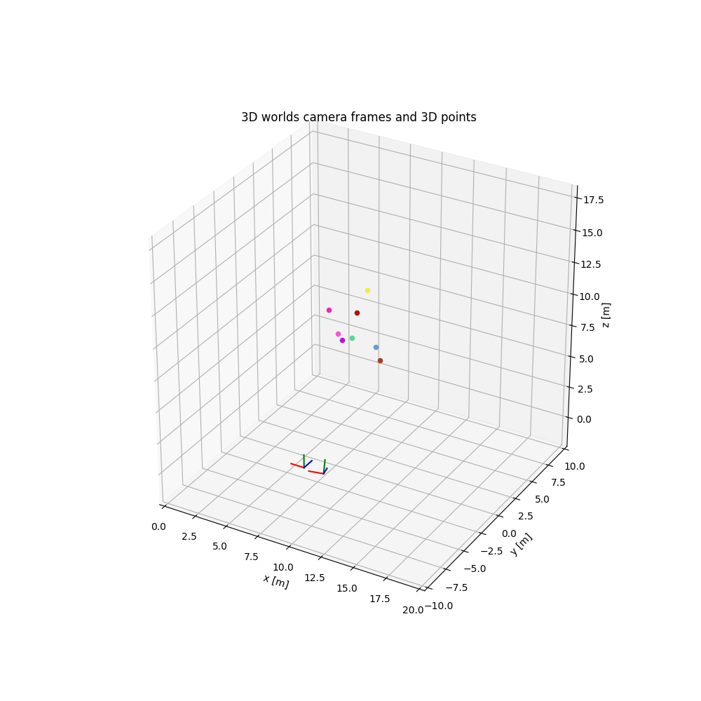
Let's have a look at a toy example using Python, full code here.
Let's generate a fixture world with two cameras and eight 3D points. In the image, each frame is represented with r (x-axis), g (y-axis) and b (z-axis).
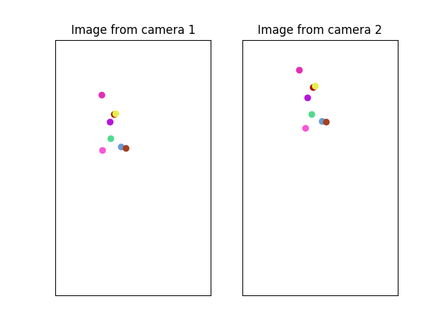
Now, we assume that our cameras have a focal length of one and we transform the points into the normalized image space. The resulting images for both the cameras are represented in the figure, where colours match point correspondences.
From the points, we can compute the Kronecker product and extract our estimated essential matrix.
def _extract_rot_transl(U, V):
    W = np.array(([0, -1, 0], [1, 0, 0], [0, 0, 1]))
    return [
        [np.dot(U, np.dot(W, V)), U[-1, :]],
        [np.dot(U, np.dot(W, V)), -U[-1, :]],
        [np.dot(U, np.dot(W.T, V)), U[-1, :]],
        [np.dot(U, np.dot(W.T, V)), -U[-1, :]],
    ]


chi = _compute_kronecker(points_1, points_2)
_, _, V1 = np.linalg.svd(chi)
F = V1[8, :].reshape(3, 3).T
U, _, V = np.linalg.svd(F)
possible_r_t = _extract_rot_transl(U, V)
Let's compare the results we got with the original rotation and translation from camera_1 to camera_2.
One of the solutions we get:
R = [[ 0.95533649, -0.        ,  0.29552021],
     [ 0.0587108 ,  0.98006658, -0.18979606],
     [-0.28962948,  0.19866933,  0.93629336]]
t = [-1.,  0.,  0.]
With the original \(R\) and \(T\):
R = [[ 0.95533649, -0.        ,  0.29552021],
     [ 0.0587108,   0.98006658, -0.18979606],
     [-0.28962948,  0.19866933,  0.93629336]]
t = [-1.5,  0.,  0.]
As you can see we were able to fully recover \(R\) and \(T\), but only up to a scaling factor.
Conclusions: We had an in-depth look at the eight-points algorithm to reconstruct the affine transformation between two camera poses observing the same 3D points. We formally introduce the algorithm, discussed caveats and we had a look at a real example using synthetic data in Python.