Is GO good at Math?

We don't usually associate GO with a language to do mathematics, geometry or deep learning. Those tasks are usually left mainly to Python.

But is GO good at math as well?

Disclaimer

This post is an effort to share my experience and knowledge about the topic. Are there languages that are a better fit for math? Yes. Is it possible to do math (at least some simple things) with GO? Yes.

Pre-requisite

To implement our code we will use gonum, which is a GO library for numerical and scientific algorithms. As a plus, it has nice plotting functions as well.

Let's have a quick look at gonum/mat, where the linear algebra libraries are implemented.

The first thing to understand about the library is that everything is done using a pointer receiver, for example:

m1 := mat.NewDense(2, 2, []float64{
    4, 0,
    0, 4,
})
m2 := mat.NewDense(2, 3, []float64{
    4, 0, 0,
    0, 0, 4,
})
var prod mat.Dense
prod.Mul(m1, m2)
fc := mat.Formatted(&prod, mat.Prefix("       "), mat.Squeeze())
fmt.Printf("prod = %v\n", fc)

The code will output:

prod = ⎡16  0   0⎤
       ⎣ 0  0  16⎦

If you see, we defined two matrices, passing the data with a slice of float64 row-major, then we created a new matrix to contain the product and then called the Mul function with the new matrix as a pointer receiver. The final part is just printing using the built-in formatter.

Let's see how to invert a matrix:

m := mat.NewDense(2, 2, []float64{
    4, 0,
    0, 4,
})
var inv mat.Dense
inv.Inverse(m)
fc := mat.Formatted(&inv, mat.Prefix("      "), mat.Squeeze())
fmt.Printf("inv = %v\n", fc)

The code will output:

inv = ⎡0.25    -0⎤
      ⎣   0  0.25⎦

Again, we defined a matrix, we created an empty matrix to contain the inverse and then we inverted the first matrix.

Solving a linear system

Let's try to solve a linear system:

\[ \begin{matrix} x + y + z = 6 \\ 2y + 5z = -4 \\ 2x + 5y - z = 27 \end{matrix} \]

This can be rewritten as \(Ax = b\)

\[ \begin{bmatrix} 4 & 1 & 1 \\ 0 & 1 & 5 \\ 2 & 7 & -1 \end{bmatrix} \begin{bmatrix} x \\ y \\ z \end{bmatrix} = \begin{bmatrix} 4 \\ -4 \\ 22 \end{bmatrix} \]

Now the solution would be \( x = A^{-1}b\) being \(A\) a square matrix with \(det \neq 0\).

Using gonum, we can either invert \(A\) or use the more generic function SolveVec, which solves a linear system.

A := mat.NewDense(3, 3, []float64{
    4, 1, 1,
    0, 1, 5,
    2, 7, -1,
})
b := mat.NewVecDense(3, []float64{4, -4, 22})
x := mat.NewVecDense(3, nil)

x.SolveVec(A, b)
fmt.Printf("%v\n", x)

Which outputs:

[0.64705 2.76470 -1.35294] 

Neural Network

Now it's time to try something a bit more complex... Let's implement a simple neural network in GO, without going too much into detail on the math (you will have to trust me on that).

Neural Networks ELI5

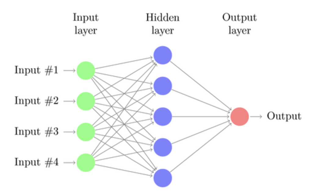
In a multilayer perceptron, you have an input, an output layer and some hidden layers. Each layer, in its simplest form, consists of a linear transformation (\(y_i = W_ix_i + b_i\), for the i-th layer) plus a nonlinear transformation called activation function (\(y_i = a_i(W_ix_i + b_i)\)). The network is trained using a cost function (\(L\)), which is a function we are trying to optimize.

For example, we have samples as inputs and outputs and we want our network to learn a function that ties the two. The cost function could be the mean squared error (MSE) between the network output given the input or the sum of the squared error (SSE) (this is really ELI5). The weights at each layer (\(W_i\)) and the biases (\(b_i\)) are our tunable parameters.

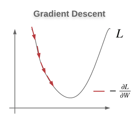
To optimize the cost function we use gradient descent: at each step, we compute the output of the network, we then compute the derivative at of the cost function with respect to the weights and biases and we update the weights in such a way that we follow the direction of the negative gradient. In principle, each step moves us closer to the minimum of the cost function.

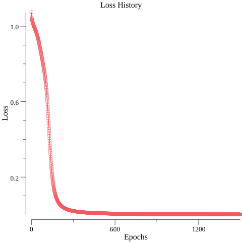
To monitor the training of our network we will be plotting the values of the loss function.

To simplify the code a bit we will assume that the network has no \(b_i\) terms. \(L = \sum (\hat(y)_y - y_i)^2\), so the SSE and our activation function is the sigmoid function (\(\sigma(x) = \frac{1}{1 + \exp(-x)} \)).

Let's see if our network can learn the toy problem in this blog post.

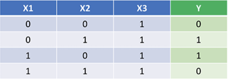
After 1,500 iterations, the output generated by the network is [0.014, 0.98, 0.98, 0.024] (the original output of the table is [0, 1, 1, 0]) which means that our simple network was able to overfit and learn the training set.

The full code can be found here.

Below you can see the plot (made with gonum/plot) of the loss during training.

One gotcha to be aware of while doing some more complex math using gonum is that chaining multiplications in which the matrices dimension change will break the dimension check even if it appears correct.

For example:

m1 := mat.NewDense(2, 3, []float64{
    0, 0, 1,
    0, 1, 1,
})

m2 := mat.NewDense(2, 3, []float64{
    1, 0, 1,
    1, 1, 1,
})

m3 := mat.NewDense(2, 3, []float64{
    0, 0, 3,
    0, 1, 1,
})

var mul mat.Dense
mul.Mul(m1, m2.T())
mul.Mul(&mul, m3)

This code will panic despite the multiplication being perfectly valid \((2\times 3)(3\times 2)(2\times 3)\). The failure happens because the auxiliary matrix you are using as a point receiver is not of the right size to contain the new multiplication.

The solution to this is to create a new auxiliary matrix for each step in which the dimension changes because of the multiplication.

var mul1 mat.Dense
mul1.Mul(m1, m2.T())
var mul2 mat.Dense
mul2.Mul(&mul1, m3)

Plotting

Plotting using gonum/plot is pretty straightforward: you can create an object of type Plot and then you add to it multiple plots using the plotutil package, which contains routines to simplify adding common plot types, such as line plots, scatter plots, etc...

As an example, to plot the loss:

p, err := plot.New()
// check error.
// ...
err = plotutil.AddLinePoints(p, "", points)
// check error.
err = p.Save(5*vg.Inch, 5*vg.Inch, "loss_history.png")
// ...

Conclusions: In this post, we explored the potential of GO to do math and linear algebra. We had a look at the gonum library, first solving a simple linear system and then implementing a simple neural network in GO. We also had a quick look at how you can use gonum to create plots.