Effective strategies for classification in CT scans

Last October I took part in the RSNA Intracranial Haemorrhage Detection Kaggle challenge. I ended up in the top 10%, which considering my full-time job and travelling, was a placement I am quite happy with.

The goal of this post is to share some ideas and strategies to work with classification in CT scans.

The task

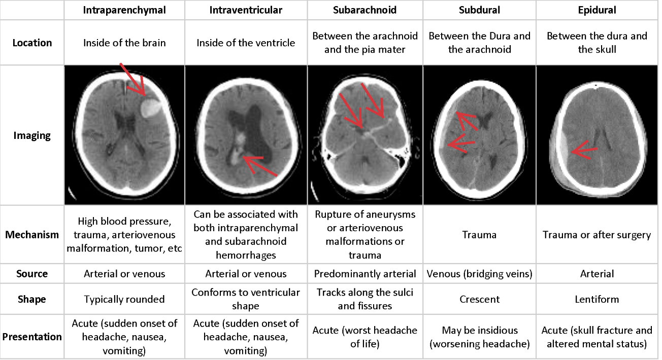
The task in this competition was to tackle a multiclass classification problem, to classify 5 different types of brain haemorrhage (a sixth class was "not present") from computerized tomography (CT) scans of patient's heads. Each type of haemorrhage tends to appear in different location of the head with different features. A summary with examples is reported below.

CT scans usually are slices on the axial plane taken at different heights. This means that you can combine consecutive scans to obtain 3D information. In general, scans are provided in the DICOM format, which is an international standard for digital medical images. DICOM files represent pixel intensities in normal units (they can range for example between -32768 and 32767 or less according to the number of bits used).

Scans

First, you can convert the scans from pixel intensities to Hounsfield Units (HU). Hounsfield Units describe a linear scale of radio intensity. Basically, values range between -1000 (radio intensity of air) and 1000 (roughly radio intensity of metal). Harder materials (such as bone or metal) will have a higher radio intensity. Lighter materials, like flesh, soft tissue or water, will have a lower radio intensity.

To convert from the DICOM to HU you usually have to look for "slope" and "intercept" in the file metadata. The two values, which are usually provided by the manufacturer allow you to get the HU:

\[ \text{scan}_{HU} = \text{scan} * \text{slope} + \text{intercept} \]

Now if you try and visualize the images in HU you will probably see something like this

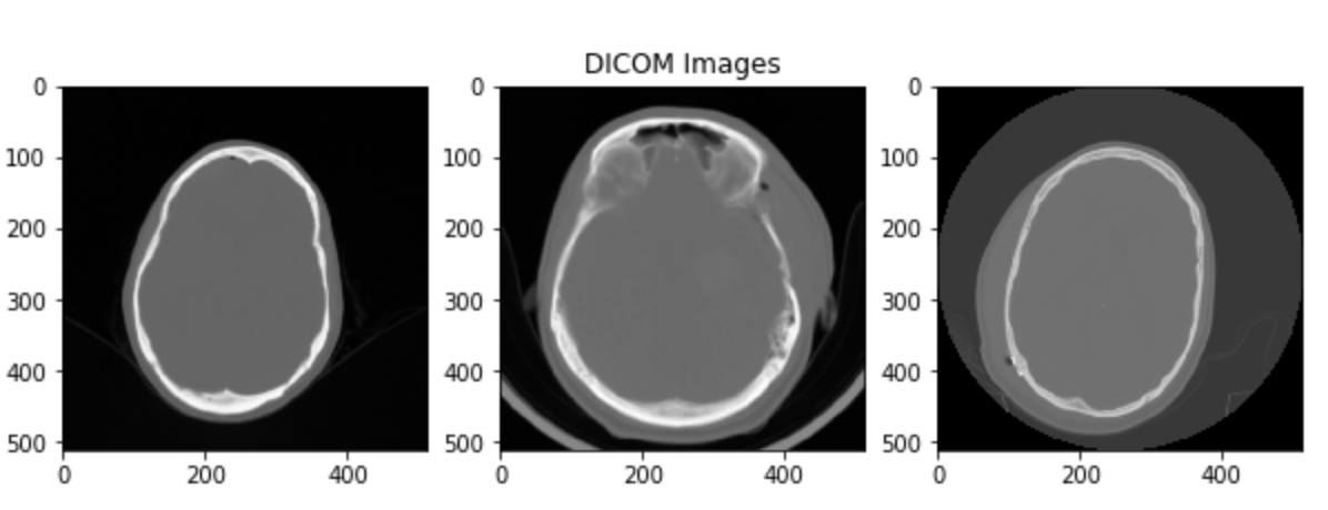
So what's the problem?

The problem is that in a normal grayscale image you can represent 256 different shades, this means that being the HU roughly 2000 values, you have 8 values per shade of grey. As a human, you cannot visually detect changes in shades that are less than 120 HU (in greyscale). That's why you don't see the nice head scans that we were expecting, but instead, you just see a grey blob.

So what do doctors do?

During scan assessment by a human doctor, what is actually done is that each scan is "focused" on a particular range of the Hounsfield Scale, giving information about a certain type of tissue. Doctors usually focus on 2-3 different windows at the same time (according to the assessment they are performing).

In the case of brain haemorrhages, there are 5 important windows, each one focusing on a type of tissue:

1. Brain Matter window: W:80 L:40
2. Blood/subdural window: W:130-300 L:50-100
3. Soft tissue window: W:350–400 L:20–60
4. Bone window: W:2800 L:600
5. Grey-white differentiation window: W:8 L:32 or W:40 L:40

The windows are expressed with two numbers W the width of the window and L the center. Each window focuses on the range:

\[ L - W / 2 < \text{HU} < L + W / 2 \]

Mimic doctors with ML

A viable approach is to choose 3 different windows and use them as the channels of a 3-channel image. In this way our network will try and learn, as a human doctor does, to classify haemorrhage using multiple windows of the same scan.

This approach works and was successfully used during the competition by lots of participants (including me). The approach is also backed up by several research papers.

Some examples of the images one obtains are shown in the pictures.

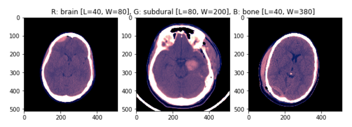
The images have been min-max scaled to then be fed to the network.

Pros

• Quite a simple approach.
• We are feeding the network the same information a human expert would use (we know it's meaningful).

Cons

• We are dropping information that the network might be able to use.

Introduce a volume component

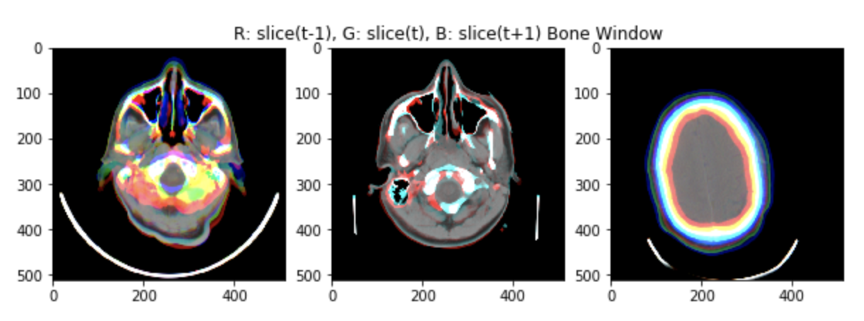
Another approach, that was quite successful in the competition was to introduce a volume component instead or together with using multiple windows.

As shown in the figure, scans are consecutive snapshots on the axial plane of the head.

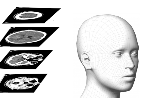
Three consecutive scans can be used as the three channels of an RGB image (using still some windowing on the Hounsfield Scale).

An example of the input images (min-max scaled) is shown in the figure.

Pros

• Quite a simple approach.
• We are now giving information to the network about volume, although limited.

Cons

• We are dropping information that the network might be able to use (for the windowing).

No windowing

An interesting approach developed during the competition was to drop windows altogether and give the network the full range of HU values. The nuance to tackle with this approach is that the distribution of the pixels over the full range is usually strongly bimodal, with values that are not evenly distributed in the whole range. The distribution can change a lot with the type of tissue that is mainly present in each scan.

A solution to this problem is to find (or craft) a nonlinear normalization function to "normalize" our data over the full range, or almost the full range.

An example can be found in the write-up of the 8th place solution to the competition.

---

Conclusions: We had a look at some possible approaches that work when dealing with classification in CT scans. We started explaining how scans work, how we can convert them to Hounsfield Units and which strategies we can use to feed the data to a neural network.