Everything you need to know about the Lucas-Kanade tracker
The Lucas-Kanade-Tomasi (LKT) tracker is one of the most used trackers in computer vision. It's easy to implement and understand, it's fast to compute and it works fairly well.
The tracker is based on the Lucas-Kanade (LK) optical flow estimation algorithm. The problem of optical flow estimation is the problem of estimating the motion of the pixels in an image across a sequence of consecutive pictures (e.g., a video).
The idea of the LK estimation is pretty straightforward.
Now, let's imagine you are observing the image from a small hole of the size of a pixel. If you know the gradient of the brightness, if you move the image, you can infer something about the direction of the movement. This is true only if the brightness cannot change for any other reasons other then motion.
We just introduced the first basic assumption of the LK tracker: the brightness of each pixel does not change in time, as each point moves in the image, it will keep it's brightness constant.
Let's exemplify with a drawing.
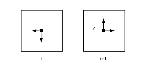
Let's assume at time t you are observing a pixel of an image (left image), and you know that the brightness is increasing towards left and down (the arrows show the gradient of the brightness). At the next time instant, after the camera moved (right image), you notice that the brightness observed through the pixel increased, given that the brightness does not change for any other reason, you can safely assume that the underlying object observed by the camera, has moved up and right (black arrows), or conversely, the camera moved with a certain velocity v down and left.
You can immediately notice one possible problem: what if the brightness doesn't change for the point we are observing? Or what if the brightness doesn't change in a certain direction?
This is called the aperture problem. You can only perceive motion in the directions that are not orthogonal to the direction of the gradient. For example, if you observe a pixel in a monochrome patch you won't be able to perceive any motion, or if you are observing a pixel on a straight edge, you cannot perceive any movement along the edge. Luckily, in natural images it's really hard to find this scenario, usually zooming to different levels will usually give you some texture with a brightness gradient in both x and y directions.
An alternative solution is to observe a window around a pixel, increasing the likelihood of a "full" brightness gradient. It is to be noted that if you use a window you are implicitly assuming that all the pixels in the window move in the same way, for this assumption to be safely made you need to have very small displacements and a properly sized window, otherwise, for complex motions you will easily break it.
Let's now have a look at the math. If you assume that the brightness (I) remains constant for each pixel (x) in time, you can write:
\[I(x(t), t) = \text{const} \Rightarrow \frac{dI}{dt} = 0\]
Applying the chain rule to compute the derivatives we get
\[\nabla I^{T}\frac{dx}{dt}+\frac{\partial I}{\partial t} = 0\]
If you observe the equation, you can see that it exactly describes the intuition we had about brightness changes and motion, and it becomes particularly clear if you rewrite it as:
\[\nabla I^{T}v = -\frac{\partial I}{\partial t}\]
where we called v the velocity of the camera motion. The equation basically says that the delta in brightness given by the velocity of the camera motion accounts for the total change of brightness in time. The velocity vector v is the unknown.
The aperture problem is clearly visible now. On the left, you have the scalar product of the gradient of the brightness and the velocity of motion. Any velocity orthogonal to the gradient will result in a null change in brightness, thus every velocity will satisfy the equation.
In the LK paper the authors proposed to solve the equation in the least square terms, that is finding the v that minimizes the equation. If we consider the case of a window (W) around the pixel x:
\[E(v) = \int_{W(x)} |\nabla I^{T}v + \frac{\partial I}{\partial t}|^{2}dx' \]
This function is quadratic in v, thus it's optimum is where the derivative is equal to zero:
\[\frac{dE}{dv} = 0 \Rightarrow v = -M^{-1}q\]
where
\[M = \int_{W(x)}\nabla I\nabla I ^{T}dx'\]
and
\[q = \int_{W(x)}\frac{\partial I(x')}{\partial t}dx'\]
As you can clearly see from the derivative expression, the matrix M which is called the structure tensor, is a 2x2 matrix. If \(det(M) = 0\), we have a patch with constant brightness, thus we are not able to solve in v, since M is not invertible. If \(det(M) = 2\) we can find v and the solution is unique. If \(det(M) = 1\) we can only find the component of v in one direction.
In the case presented, we are estimating motion given only by translation, the math can be simply modified to estimate an affine transformation (rotation plus translation) in the following way
\[E(v) = \int_{W(x)} |\nabla I^{T}S(x')p + \frac{\partial I}{\partial t}|^{2}dx' \]
where the affine transformation is modeled with a parametric model:
\[S(x)p = \begin{pmatrix} x & y& 1&0&0&0\\ 0 &0&0&x&y&1 \end{pmatrix}\begin{pmatrix} p1&p2&p3&p4&p5&p6\\ \end{pmatrix}^{T}\]
Now we can easily solve \(dE/dp = 0\).
Let's see an example using OpenCV and Python (you can find the full code here).
video = cv2.VideoCapture(input_video)
success, frame = video.read()
previous_frame_gray = cv2.cvtColor(frame, cv2.COLOR_BGR2GRAY)
previous_points = cv2.goodFeaturesToTrack(previous_frame_gray, **DEFAULT_FEATURES_PARAMS)
First we open the video stream, read the first frame and find pixels to track. OpenCV provides the function goodFeaturesToTrack. Under the hood, the function finds the most prominent corners of the image using the Shi-Tomasi corner detector.
If you had to do it in practice, a simple way to identify good points is to compute the matrix M for all the pixels in the image and choose a set of points for which \(det(M)\) is greater than a certain threshold.
An alternative is to use the Harris corner detector. The idea is to weight the matrix M with a Gaussian centred on the window W centre
\[M = G_{\sigma}\nabla I \nabla I ^{T}\]
and then choose pixels such that
\[C(x) = det(M) + k*tr^{2}(M) > \vartheta \]
Intuitively, the eigenvectors of M tell the direction of maximum and minimum variation of the brightness, while the eigenvalues tell the amount of variation. In particular, if the eigenvalues are both low we are in a flat region (there is not much change in gradient), if one of the eigenvalues is bigger then the other we are on an edge, and if both the eigenvalues are high, we are probably on a corner (brightness changes in both the directions).
The Gaussian improves the results, weighting M based on the distance from the centre.
Now, if you remember from linear algebra
\[C(x) = det(M) + k*tr^{2}(M) = \lambda_1 \lambda_2 + k(\lambda_1+\lambda_2)^{2}\]
so the criteria that we are using to choose the points will yield a higher value if both the eigenvalues are high.
In OpenCV, you can specify to use the Harris detector (you can check in the code how).
Once we found the first interesting points, we can just iteratively extract a new frame and use the LK tracker to compute the optical flow.
success, frame = video.read()
frame_gray = cv2.cvtColor(frame, cv2.COLOR_BGR2GRAY)
new_points, st, _ = cv2.calcOpticalFlowPyrLK(previous_frame_gray,
                                             frame_gray,
                                             previous_points,
                                             None,
                                             **DEFAULT_LK_PARAMS)
That's what the results look like:

If you check the full code you will notice that the LK tracker has some termination criteria argument. This is interesting because we didn't talk about LK being an iterative algorithm (you iterate on the frames but you do not iterate on each frame). The parameter is used because OpenCV uses a more robust version of LK, which uses "pyramids". One of the main assumptions of the LK algorithm is that we are dealing with very small motions (~1 pixel) and this is never the case, especially with high-res cameras. A solution is to use a coarse to fine approach (a sort of resolution pyramid). We start making the image more coarse (bigger pixels will result in smaller motions) and compute the tracking after we estimated the flow at a coarser scale, we then make the image finer and go on iteratively at higher and higher levels of resolution.
Conclusions: We had an in-depth look at the Lucas-Kanade tracker to estimate the optical flow from a sequence of images. We introduced the Harris corner detector and we had a look at a real-life example using OpenCV.